© 2022. All rights reserved.
© 2022. All rights reserved.
Duo Han, Yilin Mo, Junfeng Wu, Sean Weerakkody, Bruno Sinopoli and Ling Shi
IEEE Transactions on Automatic Control, To be appeared
Link to the paper
If you want to leave any comments, you can annotate the pdf. I will try to be responsive. You can also annotate this page or leave comments below.
We propose an open-loop and a closed-loop stochastic event-triggered sensor schedule for remote state estimation. Both schedules overcome the essential difficulties of existing schedules in recent literature works where, through introducing a deterministic event-triggering mechanism, the Gaussian property of the innovation process is destroyed which produces a challenging nonlinear filtering problem that cannot be solved unless approximation techniques are adopted. The proposed stochastic event-triggered sensor schedules eliminate such approximations. Under these two schedules, the minimum mean squared error (MMSE) estimator and its estimation error covariance matrix at the remote estimator are given in a closed-form. The stability in terms of the expected error covariance and the sample path of the error covariance for both schedules is studied. We also formulate and solve an optimization problem to obtain the minimum communication rate under some estimation quality constraint using the open-loop sensor schedule. A numerical comparison between the closed-loop MMSE estimator and a typical approximate MMSE estimator with deterministic event-triggered sensor schedule, in a problem setting of target tracking, shows the superiority of the proposed sensor schedule.
The code is written in Matlab R2009b (7.9.0.529) with the following dependency
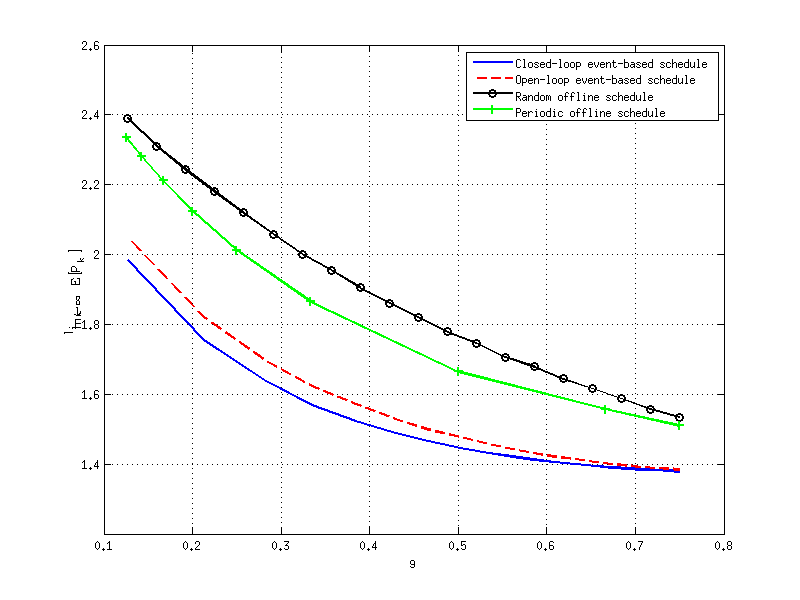
%Compare the periodic schedule, the closed-loop schedule, the open loop
%schedule and the random schedule.

close all;
clear all;
clc;

%%%% Since there is no close-form relationship between rate and  Z.
%%%% we need to find the empirical mapping from rate to Z.

% parameter setting
n = 1;
m = 1;
A = 0.8; % generate a stable A
C = 1;
Q = 1*eye(n);
sqrtQ = sqrtm(Q);
R = 1*eye(m);
sqrtR = sqrtm(R);

N = 40000;
sample = 20; % x-axis data points

Px = dlyap(A,Q);      %asymptotic covariance of x
Py = C * Px * C' + R; %asymptotic covariance of y


Z_data = zeros(1,sample);
Z_data(1)=0.01;
Z_data(2)=0.04;
Z_data(3)=0.09;

for i=1:sample
    Z_data(i)=exp(0.1*i)-1; %generates uniform Z data points
end


j=0;
h = waitbar(0,'please wait...');

rate=zeros(1,sample);
close_empiricalrate_data = zeros(1,n);
close_empiricalmse_data = zeros(1,n);
open_empiricalrate_data = zeros(1,n);
open_empiricalmse_data = zeros(1,n);
periodic_empiricalrate_data = zeros(1,n);
periodic_empiricalmse_data = zeros(1,n);
periodic_rate = zeros(1,n);
random_empiricalrate_data = zeros(1,n);
random_empiricalmse_data = zeros(1,n);
jf_empiricalrate_data = zeros(1,n);
jf_empiricalmse_data = zeros(1,n);

for i=1:sample

    %timer update
    j=j+1;
    waitbar(j/sample,h);


    x=zeros(1,N+1);
    Sigma = eye(n);
    x(1) = sqrtm(Sigma)*randn(1,n);

    y=zeros(1,N+1);

    Z = Z_data(i);
    invZ = 1/Z;


    close_empiricalmse = zeros(n); %average error*error'
    close_mse = zeros(n); %average P_k
    close_empiricalrate = 0;

    open_empiricalmse = zeros(n);
    open_mse = zeros(n);
    open_empiricalrate = 0;

    periodic_empiricalmse = zeros(n);
    periodic_mse = zeros(n);

    random_empiricalmse = zeros(n);
    random_mse = zeros(n);

    for k=1:N  %linear dynamic system
	x(k+1) = A * x(k) + sqrtQ * randn(1,n);
	y(k) = C * x(k) + sqrtR * randn(1,m);
    end

    %% closed-loop event-based MMSE under different rate
    hatx = zeros(1,n);
    P = Sigma;

    for k = 1:N


	%generate a uniform random variable
	zeta = rand();
	threshold = exp(-0.5*(y(k)-C*hatx)'*(Z)*(y(k)-C*hatx));
	if zeta < threshold % not send y
	    F = P * C' / ( C*P*C' + R + invZ);
	    hatx = hatx;
	    P = P - F*C*P;
	else % send y
	    L = P * C' / ( C*P*C' + R);
	    hatx = (eye(n) - L*C)*hatx + L*y(k);
	    P = P - L*C*P;
	    close_empiricalrate = close_empiricalrate + 1;
	end
	%prediction step
	hatx = A * hatx;
	P = A * P * A' + Q;
	close_mse = close_mse + P;
	close_error = x(k) - hatx;
	close_empiricalmse = close_empiricalmse + close_error * close_error';
    end

    close_mse_data(i)=close_mse / N;
    close_empiricalmse_data(i) = close_empiricalmse / N;
    close_empiricalrate_data(i) = close_empiricalrate / N;

    %% open-loop event-based MMSE under different rate

    Y = ((1/(1-close_empiricalrate_data(i)))^2-1)/Py; % compute Y according to the empirical rate in the closed-loop case

    hatx = zeros(1,n);
    P = Sigma;

    for k = 1:N
	%prediction step

	%uniform random variable
	zeta = rand();
	threshold = exp(-0.5*y(k)'*Y*y(k));
	if zeta < threshold % not send y
	    L = P * C' / ( C*P*C' + R + 1/Y);
	    hatx = (eye(n) - L*C)*hatx;
	    P = P - L*C*P;
	else % send y
	    L = P * C' / ( C*P*C' + R);
	    hatx = (eye(n) - L*C)*hatx + L*y(k);
	    P = P - L*C*P;
	end
	hatx = A * hatx;
	P = A * P * A' + Q;
	open_mse = open_mse + P;
	open_error = x(k) - hatx;
	open_empiricalmse = open_empiricalmse + open_error * open_error';
    end

    open_mse_data(i)=open_mse / N;
    open_empiricalmse_data(i) = open_empiricalmse / N;

    %% periodic offline MMSE under different rate
    hatx = zeros(1,n);
    P = Sigma;

    if i<sample/2
	for a=1:N
	    if mod(a,i+1)==1 % send y
		L = P * C' / ( C*P*C' + R);
		hatx = (1 - L*C)*hatx + L*y(a);
		P = P - L*C*P;
	    else % not send y
		hatx = hatx;
		P = P;
	    end
	    hatx = A * hatx;
	    P = A * P * A' + Q;
	    periodic_mse = periodic_mse + P;
	end
    else
	for a=1:N

	    if mod(a,i-sample/2+3)==1 % not send y
		hatx = hatx;
		P = P;
	    else % send y
		L = P * C' / ( C*P*C' + R);
		hatx = (1 - L*C)*hatx + L*y(a);
		P = P - L*C*P;
	    end
	    hatx = A * hatx;
	    P = A * P * A' + Q;
	    periodic_mse = periodic_mse + P;
	end
    end
    if i<sample/2
	periodic_rate(sample/2-i)=1/(i+1);
	periodic_mse_data(sample/2-i)=periodic_mse / N;
    else
	periodic_rate(i)=1-1/(i-sample/2+3);
	periodic_mse_data(i)=periodic_mse / N;
    end
end

rate_rand=zeros(1,sample);
rate_rand=[close_empiricalrate_data(1):(close_empiricalrate_data(sample)-close_empiricalrate_data(1))/19:close_empiricalrate_data(sample)];


for i=1:sample
    random_empiricalmse = zeros(n);
    random_mse = zeros(n);
    %% random offline MMSE under different rate
    hatx = zeros(1,n);
    P = Sigma;

    for k = 1:N

	if zeta < 1-rate_rand(i) % not send y
	    hatx = hatx;
	    P = P;
	else % send y
	    L = P * C' / ( C*P*C' + R);
	    hatx = (eye(n) - L*C)*hatx + L*y(k);
	    P = P - L*C*P;
	end
	%prediction step
	hatx = A * hatx;
	P = A * P * A' + Q;
	zeta = rand();
	random_mse = random_mse + P;
	random_error = x(k) - hatx;
	random_empiricalmse = random_empiricalmse + random_error * random_error';
    end

    random_mse_data(i)=random_mse / N;
    random_empiricalmse_data(i) = random_empiricalmse / N;

end

%%% plot the figures
close(h);
figure;
plot(close_empiricalrate_data,close_mse_data,'LineWidth',2);
hold on;
plot(close_empiricalrate_data,open_mse_data, 'r--','LineWidth',2);
hold on;
plot(rate_rand,random_mse_data,'k-o','LineWidth',2);
hold on;
plot(periodic_rate(3:sample-9),periodic_mse_data(3:sample-9),'g-+','LineWidth',2);
% hold on;
% plot(close_empiricalrate_data,jf_mse_data,'m-*','LineWidth',2);
legend('Closed-loop event-based schedule','Open-loop event-based schedule','Random offline schedule','Periodic offline schedule');
xlabel('\gamma');
ylabel('$\lim_{k\rightarrow\infty}\rm E[P_k^-]$','Interpreter','LaTex');
%ylabel('lim_{k\rightarrow \infty} E[P_k^-]');
grid on;

filename = '../../../public/tac-13-2.png';
print('-dpng', filename, '-r100');
ans = filename % return the filename to org-mode
% plot the upper bound, the lower bound and the empirical expected error of
% covariance of the open loop schedule
close all;
clear all;
n = 2;
m = 1;
A = [0.8 1;0 0.95]; % generate a stable A
C = [1 1];
Q = eye(n);
sqrtQ = sqrtm(Q);
R = eye(m);
sqrtR = sqrtm(R);
N = 50000;
sample = 30; % x-axis data points
Px = dlyap(A,Q); %asymptotic covariance of x
Py = C * Px * C' + R; %asymptotic covariance of y
j=0;
h = waitbar(0,'please wait...');
rate=zeros(1,sample);
open_empiricalrate_data = zeros(1,sample);
open_empiricalmse_data = zeros(1,sample);
test_mse_data = zeros(1,sample);
seq = zeros(1,N);
%% open-loop event-based MMSE under different rate
for i=1:sample
j=j+1;
waitbar(j/sample,h);
rate(i)=0.001+i/sample*0.9;
Y = ((1/(1-rate(i)))^2-1)/Py; % compute Y according to the rate
x=zeros(n,N+1);
Sigma = eye(n);
x(:,1) = sqrtm(Sigma)*randn(n,1);
y=zeros(m,N+1);
open_empiricalmse = zeros(n); %average error*error'
open_mse = zeros(n); %average P_k
open_empiricalrate = 0;
upper_mse = zeros(n); %average P_k
lower_mse = zeros(n); %average P_k
hatx = zeros(n,1);
P = Sigma;
for k = 1:N
L = P * C' / ( C*P*C' + R +1/Y);
hatx = (eye(n) - L*C)*hatx + L*y(:,k);
P = P - L*C*P;
%prediction step
hatx = A * hatx;
P = A * P * A' + Q;
upper_mse = upper_mse + P;
end
upper_mse_data(i)=trace(upper_mse) / N;
hatx = zeros(n,1);
P = Sigma;
for k = 1:N
L = P * C' / ( C*P*C' + 1/(rate(i)/R + (1-rate(i))/(R+1/Y)) );
hatx = (eye(n) - L*C)*hatx + L*y(:,k);
P = P - L*C*P;
%prediction step
hatx = A * hatx;
P = A * P * A' + Q;
lower_mse =lower_mse + P;
end
lower_mse_data(i)=trace(lower_mse) / N;
hatx = zeros(n,1);
P = Sigma;
for k=1:N %linear dynamic system
x(:,k+1) = A * x(:,k) + sqrtQ * randn(n,1);
y(:,k) = C * x(:,k) + sqrtR * randn(m,1);
end
for k = 1:N
%uniform random variable
zeta = rand();
threshold = exp(-0.5*y(:,k)'*Y*y(:,k));
if zeta < threshold % not send y
L = P * C' / ( C*P*C' + R + 1/Y);
hatx = (eye(n) - L*C)*hatx;
P = P - L*C*P;
seq(k) = 0;
else % send y
L = P * C' / ( C*P*C' + R);
hatx = (eye(n) - L*C)*hatx + L*y(:,k);
P = P - L*C*P;
seq(k) = 1;
end
%prediction step
hatx = A * hatx;
P = A * P * A' + Q;
open_mse = open_mse + P;
open_error = x(:,k) - hatx;
open_empiricalmse = open_empiricalmse + open_error * open_error';
end
open_mse_data(i)=trace(open_mse) / N;
open_empiricalmse_data(i) = trace(open_empiricalmse) / N;
end
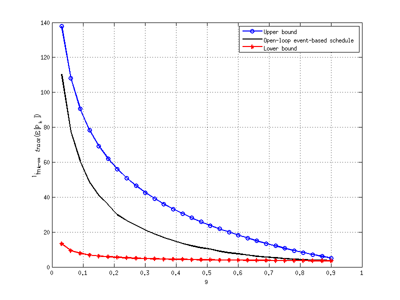
close(h);
figure;
plot(rate,upper_mse_data, 'b-o','LineWidth',2);
hold on;
plot(rate,open_mse_data, 'k-','LineWidth',2);
hold on;
plot(rate,lower_mse_data, 'r-*','LineWidth',2);
hold on;
legend('Upper bound','Open-loop event-based schedule','Lower bound');
ylabel('$\lim_{k\rightarrow\infty}trace(\rm E[P_k^-])$','Interpreter','LaTex');
xlabel('\gamma');
%h = legend;
%set(h, 'interpreter', 'latex');
grid on;
filename = '../../../public/tac-13-3.png';
print('-dpng', filename, '-r100');
ans = filename % return the filename to org-mode
% plot the upper bound, the lower bound and the empirical expected error of
% covariance of the closed loop schedule
close all;
clear all;
% parameter setting
n = 2;
m = 1;
A = [1.001 1;0 0.95]; % generate an unstable A
C = [1 1];
Q = eye(n);
sqrtQ = sqrtm(Q);
R = eye(m);
sqrtR = sqrtm(R);
N = 5000;
sample2=20;
j=0;
h = waitbar(0,'please wait...');
Z_data = zeros(1,sample2);
% for i=1:sample2
% Z_data(i)=0.1+9.9*(i-1)/sample2; %generates uniform Z data points
% end
Z_data = 0.1*[0.1 0.15 0.2 0.3 0.5 0.8 1.3 1.8 2.9 3.5 4.3 5.2 6.3 7.4 8.5 9.6 10.7 11.8 12.9 150];
rate=zeros(1,sample2);
close_empiricalrate_data = zeros(1,sample2);
close_empiricalmse_data = zeros(1,sample2);
close_mse_data=zeros(1,sample2);
upper_mse_data=zeros(1,sample2);
lower_mse_data=zeros(1,sample2);
%% close-loop event-based MMSE under different rate
for i=1:sample2
%timer update
j=j+1;
waitbar(j/sample2,h);
x=zeros(n,N+1);
Sigma = eye(n);
x(:,1) = sqrtm(Sigma)*randn(n,1);
y=zeros(m,N+1);
close_empiricalmse = zeros(n); %average error*error'
close_mse = zeros(n); %average P_k
close_empiricalrate = 0;
hatx = zeros(n,1);
P = Sigma;
for k=1:N %linear dynamic system
x(:,k+1) = A * x(:,k) + sqrtQ * randn(n,1);
y(:,k) = C * x(:,k) + sqrtR * randn(m,1);
end
Z = Z_data(i);
invZ = 1/Z;
for k = 1:N
%uniform random variable
zeta = rand();
threshold = exp(-0.5*(y(:,k)-C*hatx)'*(Z)*(y(:,k)-C*hatx));
if zeta < threshold % not send y
F = P * C' / ( C*P*C' + R + invZ);
hatx = hatx;
P = P - F*C*P;
else % send y
L = P * C' / ( C*P*C' + R);
hatx = (eye(n) - L*C)*hatx + L*y(:,k);
P = P - L*C*P;
close_empiricalrate = close_empiricalrate + 1;
end
%prediction step
hatx = A * hatx;
P = A * P * A' + Q;
close_mse = close_mse + P;
close_error = x(:,k) - hatx;
close_empiricalmse = close_empiricalmse + close_error * close_error';
end
close_mse_data(i) = trace(close_mse) / N;
close_empiricalmse_data(i) = trace(close_empiricalmse) / N;
close_empiricalrate_data(i) = trace(close_empiricalrate) / N;
upper_mse = zeros(n); %average P_k
hatx = zeros(n,1);
P = Sigma;
for k = 1:N
L = P * C' / ( C*P*C' + R +1/Z);
hatx = (eye(n) - L*C)*hatx + L*y(:,k);
P = P - L*C*P;
%prediction step
hatx = A * hatx;
P = A * P * A' + Q;
upper_mse = upper_mse + P;
end
upper_mse_data(i)=trace(upper_mse) / N;
upper_gamma= 1-1/sqrt(1+(C*upper_mse*C'/N+R)*Z);
%upper_gamma= 1-1/sqrt(1+(C*C*0.5781+R)*Z);
lower_mse = zeros(n); %average P_k
Sigma = eye(n);
hatx = zeros(n,1);
P = Sigma;
for k = 1:N
L = P * C' / ( C*P*C' + 1/(upper_gamma/R + (1-upper_gamma)/(R+1/Z)) );
%L = P * C' / ( C*P*C' + R );
hatx = (eye(n) - L*C)*hatx + L*y(:,k);
P = P - L*C*P;
%prediction step
hatx = A * hatx;
P = A * P * A' + Q;
lower_mse =lower_mse + P;
end
lower_mse_data(i)=trace(lower_mse) / N;
end
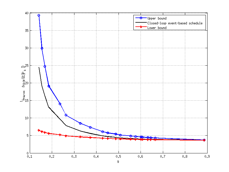
close(h);
figure;
plot(close_empiricalrate_data,upper_mse_data, 'b-o','LineWidth',2);
hold on;
plot(close_empiricalrate_data,close_mse_data, 'k-','LineWidth',2);
hold on;
plot(close_empiricalrate_data,lower_mse_data, 'r-*','LineWidth',2);
legend('Upper bound','Closed-loop event-based schedule','Lower bound');
ylabel('$\lim_{k\rightarrow\infty}trace(\rm E[P_k^-])$','Interpreter','LaTex');
xlabel('\gamma');
%h = legend;
%set(h, 'interpreter', 'latex');
grid on;
filename = '../../../public/tac-13-4.png';
print('-dpng', filename, '-r100');
ans = filename % return the filename to org-mode
m = 2; n = 2;
A=[0.8 1;0 0.95];
C=[0.5 0.3; 0 1.4];
Q = eye(n);
inQ = inv(Q);
R = eye(n);
inR = inv(R);
L = chol(R);
I = eye(n);
subrate=zeros(1,50);
kappa=zeros(1,50);
lbound=zeros(1,50);
[XX,YY,ZZ]=dare(A',C',Q,R,zeros(n),eye(n));
for i=3:50
Delta=XX+0.02*i*eye(n);
invDelta=inv(Delta);
Px = dlyap(A,Q); %asymptotic covariance of x
Pi = C * Px * C' + R; %asymptotic covariance of y
PU = chol(Pi);
lgPi = log(det(Pi));
lginvR = log(det(inv(R)));
invPi = inv(Pi);
%constant = log((1-rate)^(-2))-lginvR-lginvR;
cvx_begin sdp
variable Y(n,n) symmetric
variable M1(n,n) symmetric
variable M2(n,n) symmetric
variable S(n,n) symmetric
minimize( trace(Pi*Y) )
subject to
[A'*inQ*A+C'*inR*C+S A'*inQ C'*inR;
inQ*A inQ-S zeros(n,m);
inR*C zeros(m,n) Y+inR]>=0
[S eye(n);
eye(n) Delta]>=0
Y>=0
-S >= -inQ
cvx_end
kappa(i)=1/sqrt(1+trace(Pi*Y))-1/sqrt(det(eye(n)+Pi*Y));
lbound(i)=1-1/sqrt(1+trace(Pi*Y));
subrate(i)=1-1/sqrt(det(eye(n)+Pi*Y));
end
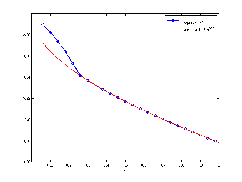
plot(0.02*(3:2:50),subrate(1,3:2:50),'b-O','linewidth',1.5);
hold on
plot(0.02*(3:50),lbound(1,3:50),'r-','linewidth',1.5)
xlabel('\varpi');
legend('Suboptimal \gamma^{Y^*}','Lower bound of \gamma^{opt}')
filename = '../../../public/tac-13-5.png';
print('-dpng', filename, '-r100');
ans = filename % return the filename to org-mode
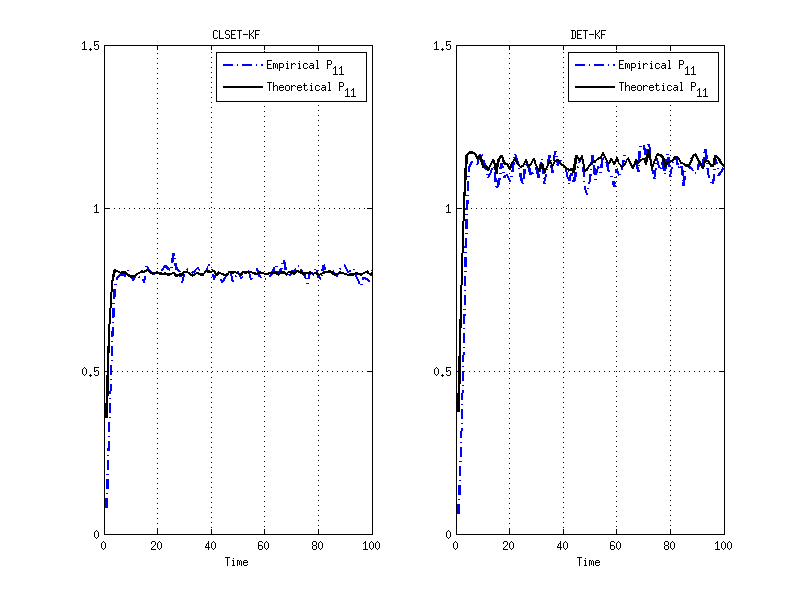
% Compare the closed-loop event-based schedule with the deterministic schedule proposed by Keyou You and Lihua Xie in [26]

% parameter setting
T = 1;
alpha = 0.01;
var_acceleration = 5;

n = 3;
A = [1 T T^2;0 1 T; 0 0 1]; % generate a stable A
m = 3;
C = eye(m);

Q = 2*alpha*var_acceleration*[(T^5)/20 (T^4)/8 (T^3)/6;(T^4)/8 (T^3)/3 (T^2)/2; (T^3)/6 (T^2)/2 T];
sqrtQ = sqrtm(Q);
R = 1*eye(m);
sqrtR = sqrtm(R);

%Z_data = 0.047*eye(m); %smaller Z, smaller rate ///for C = eye(3)
%delta_data = [4.30]; %smaller delta, larger rate///for C = eye(3)
Z_data = 0.52*eye(m); %smaller Z, smaller rate ///for C = eye(3)
delta_data = [1.6]; %smaller delta, larger rate///for C = eye(3)

N = 100;
sample2=1;
countermax=5000;


j=0;
h = waitbar(0,'please wait...');


% for i=1:sample2
%     Z_data(i)=0.1+9.9*(i-1)/sample2; %generates uniform Z data points
% end

rate=zeros(1,sample2);
close_empiricalrate_data = zeros(1,sample2);
close_empiricalmse_data = zeros(1,sample2);
close_mse_data=zeros(1,sample2);
close_hatx_data=zeros(n,N+1);
close_P_data=zeros(1,N);
close_empiricalP_data=zeros(1,N);

keyou_empiricalrate_data = zeros(1,sample2);
keyou_empiricalmse_data = zeros(1,sample2);
keyou_mse_data=zeros(1,sample2);
keyou_hatx_data=zeros(n,N+1);
keyou_P_data=zeros(1,N);
keyou_empiricalP_data=zeros(1,N);

Sigma = 0.1*[1 1/T 0;1/T 2/(T^2) 0; 0 0 0.00001];

%% close-loop event-based MMSE under different rate
for counter=1:countermax
	% timer update
	j=j+1;
	waitbar(j/countermax,h);

	x(:,1) = sqrtm(Sigma)*randn(n,1);

	% generate linear dynamic system
	x=zeros(n,N+1);
	y=zeros(m,N+1);

	for k=1:N
	    x(:,k+1) = A * x(:,k) + sqrtQ * randn(n,1);
	    y(:,k) = C * x(:,k) + sqrtR * randn(m,1);
	end

	hatx = zeros(n,1);
	P = Sigma;

	close_empiricalmse = zeros(n); %average error*error'
	close_mse = zeros(n); %average P_k
	close_empiricalrate = 0;

      %%%%%%%%%%% proposed closed loop scheduler    %%%%%%%%%%%%%%%%%%%%%%%%%
	Z = Z_data;
	invZ = inv(Z);

	for k = 1:N

	    %prediction step
	    hatx = A * hatx;
	    P = A * P * A' + Q;

	    %generate a uniform random variable
	    zeta = rand();
	    threshold = exp(-0.5*(y(:,k)-C*hatx)'*(Z)*(y(:,k)-C*hatx));
	    if zeta < threshold % not send y
		F = P * C' / ( C*P*C' + R + invZ);
		hatx = hatx;
		P = P - F*C*P;
	    else % send y
		L = P * C' / ( C*P*C' + R);
		hatx = (eye(n) - L*C)*hatx + L*y(:,k);
		P = P - L*C*P;
		close_empiricalrate = close_empiricalrate + 1;
	    end

	    close_mse = close_mse + P;
	    close_error = x(:,k) - hatx;
		%close_P_data(:,k) = close_P_data(:,k) + trace(P);
	    close_P_data(:,k) = close_P_data(:,k) + P(1,1);
	    temp1 = close_error * close_error';
	    close_empiricalP_data(:,k) = close_empiricalP_data(:,k) + temp1(1,1);
		%close_empiricalP_data(:,k) = close_empiricalP_data(:,k) + trace(temp1);

	end

	%close_mse_data = close_mse(1,1) / N;
	close_mse_data = trace(close_mse) / N;
	%close_empiricalmse_data = close_empiricalmse_data(i)+close_empiricalmse(1,1) / N;
	close_empiricalmse_data = close_empiricalmse_data+trace(close_empiricalmse) / N;
	%close_empiricalrate_data = close_empiricalrate_data + close_empiricalrate(1,1) / N;
	close_empiricalrate_data = close_empiricalrate_data + trace(close_empiricalrate) / N;

	%%%%%%%%% keyou's scheduler %%%%%%%%%%%%%%%%%%%%%
	hatx = zeros(n,1);
	P = Sigma;

	keyou_empiricalmse = zeros(n); %average error*error'
	keyou_mse = zeros(n); %average P_k
	keyou_empiricalrate = 0;

	delta = delta_data;

	for k = 1:N

	    %prediction step
	    hatx = A * hatx;
	    P = A * P * A' + Q;

	    zk = inv(sqrt(C*P*C'+R))*(y(:,k)-C*hatx);
	    if abs(zk) < delta % not send y
		L = P * C' / ( C*P*C' + R);
		hatx = hatx;
		hx = sqrt(2/pi)*delta*exp(-(delta^2)/2)/(1-erfc(delta/sqrt(2)));
		P = P - hx*L*C*P;
	    else % send y
		L = P * C' / ( C*P*C' + R);
		hatx = (eye(n) - L*C)*hatx + L*y(:,k);
		P = P - L*C*P;
		keyou_empiricalrate = keyou_empiricalrate + 1;
	    end

	    keyou_mse = keyou_mse + P;
	    keyou_error = x(:,k) - hatx;
	    keyou_empiricalmse = keyou_empiricalmse + keyou_error * keyou_error';

	    keyou_hatx_data(:,k) = hatx;
	    keyou_P_data(:,k) = keyou_P_data(:,k) + P(1,1);
	       %keyou_P_data(:,k) = keyou_P_data(:,k) + trace(P);
	    temp2 = keyou_error * keyou_error';
	    keyou_empiricalP_data(:,k) = keyou_empiricalP_data(:,k) + temp2(1,1);
		%keyou_empiricalP_data(:,k) = keyou_empiricalP_data(:,k) + trace(temp2);

	end

	%keyou_mse_data(i) = keyou_mse(1,1) / N;
	keyou_mse_data = trace(keyou_mse) / N;
	%keyou_empiricalmse_data(i) = keyou_empiricalmse_data(i)+ keyou_empiricalmse(1,1) / N;
	keyou_empiricalmse_data = keyou_empiricalmse_data+ trace(keyou_empiricalmse) / N;
	%keyou_empiricalrate_data = keyou_empiricalrate_data + keyou_empiricalrate(1,1)/ N;
	keyou_empiricalrate_data = keyou_empiricalrate_data + trace(keyou_empiricalrate)/ N;
end

close_P_data = close_P_data/countermax;
close_empiricalP_data = close_empiricalP_data/countermax;
close_empiricalrate_data= close_empiricalrate_data/countermax;
keyou_P_data = keyou_P_data/countermax;
keyou_empiricalP_data = keyou_empiricalP_data/countermax;
keyou_empiricalrate_data = keyou_empiricalrate_data/countermax;


Keyou_rate=keyou_empiricalrate_data
Mine_rate=close_empiricalrate_data
close(h);
figure;
subplot(1,2,1);
plot(1:N,close_empiricalP_data, 'b-.','LineWidth',2);
hold on;
plot(1:N,close_P_data, 'k-','LineWidth',2);
title('CLSET-KF');
legend('Empirical P_{11}','Theoretical P_{11}');
xlabel('Time');
axis([0 N 0 1.5]); % for high rate
%axis([0 N 0 30]); % for low rate
grid on;
subplot(1,2,2);
plot(1:N,keyou_empiricalP_data, 'b-.','LineWidth',2);
hold on;
plot(1:N,keyou_P_data, 'k-','LineWidth',2);
title('DET-KF');
legend('Empirical P_{11}','Theoretical P_{11}');
xlabel('Time');
axis([0 N 0 1.5]);% for high rate
%axis([0 N 0 30]);% for low rate
grid on;

filename = '../../../public/tac-13-6.png';
print('-dpng', filename, '-r100');
ans = filename % return the filename to org-mode