
Model Reference Adaptive Control
01 Sep 2015Consider the following first-order linear system:
\begin{equation} \dot{x} = a x + bu, \label{eq:truesystem} \end{equation}where \(a,\,b\) are unknown parameters. However, the sign of \(b\) is known.
Suppose that we want the linear system \eqref{eq:truesystem} to track the following reference system:
\begin{equation} \dot{x_m} = a_m x_m + b_m r, \label{eq:refsystem} \end{equation}where \(a_m < 0\) and \(b_m\) are known and \(r(t)\) is a known reference signal.
Suppose we use the following control law:
\begin{equation} u = \hat k_x x + \hat k_r r. \end{equation}Then the dynamic of system \eqref{eq:truesystem} will be
\begin{equation} \dot{x} = (a + b \hat k_x) x + b \hat k_r r. \end{equation}Therefore, if we can make
\begin{equation} \hat k_x = k_x \triangleq \frac{a_m-a}{b}\text{ and }\hat k_r = k_r \triangleq \frac{b_m}{b}, \end{equation}then the dynamic of system \eqref{eq:truesystem} will follow the reference system. Let us denote \(\Delta k_x \triangleq k_x - \hat k_x\) and \(\Delta k_r \triangleq k_r - \hat k_r\).
Now consider the dynamic of the error \(e \triangleq x - x_m\), we have
\begin{align*} \dot{e}& = (a + b \hat k_x) x + b \hat k_r r - a_m x_m - b_m r\\ & = a_m(x - x_m) - b \Delta k_x x - b \Delta k_r r \\ & = a_m e - b \Delta k_x x - b \Delta k_r r . \end{align*}Therefore, if we consider the following candidate Lyapunov function
\begin{equation} V = \frac{1}{2}\left(e^2 + |b|(\gamma_x^{-1} \Delta k_x^2 + \gamma_r^{-1} \Delta k_r^2)\right), \end{equation}where \(\gamma_x,\,\gamma_r > 0\). Then we have
\begin{align*} \dot{V} = a_m e^2 &- |b|\Delta k_x \left(\text{sgn}(b)ex + \gamma_x^{-1}\dot{\hat k_x}\right) \\ &- |b|\Delta k_r \left(\text{sgn}(b)er + \gamma_r^{-1}\dot{\hat k_r}\right). \end{align*}Therefore, if we use the following update rule on \(\hat k_x\) and \(\hat k_r\):
\begin{equation} \dot{\hat k_x} = -\gamma_x \text{sgn}(b) ex\text{ and }\dot{\hat k_r} = -\gamma_r \text{sgn}(b) er,\\ \end{equation}then \(\dot{V} = a_m e^2 \leq 0\). One can then prove that \(\ddot{V} =2 a_m e \dot{e}\) is bounded and thus \(\lim_{t\rightarrow\infty} \dot{V} = 0\) and hence \(e \rightarrow 0\).
Simulation
Assume that the system is given as
\begin{equation} \dot{x} = x + u, \end{equation}while we want the system to tract the following system:
\begin{equation} \dot{x_m} = - x_m + r = - x_m + \sin(t). \end{equation}import numpy as np import matplotlib import matplotlib.pyplot as plt import seaborn as sns # for the sake of appreances from scipy.integrate import odeint a = 1. b = 1. am = -1. bm = 1. gammax = 10. gammar = 10. # y is a vector of [x ,x_m, \hat k_x, \hat k_r] def f(y, t): x = y[0] xm = y[1] hatkx = y[2] hatkr = y[3] r = np.sin(t) e = x - xm u = hatkx * x + hatkr * r f0 = a * x + b * u f1 = am * xm + bm * r f2 = -1 * gammax * e * x f3 = -1 * gammar * e * r return [f0, f1, f2, f3] t = np.linspace(0, 20., 10000) x0 = 0. xm0 = 0. hatkx0 = 0. hatkr0 = 0. y0 = [x0, xm0, hatkx0, hatkr0] solution = odeint(f, y0, t) x = solution[:, 0] xm = solution[:, 1] hatkx = solution[:, 2] hatkr = solution[:, 3] fig = plt.figure() plt.rc('text', usetex=True) plt.plot(t, np.sin(t), label=r'$r(t)$') plt.plot(t, x, label=r'$x(t)$') plt.plot(t, xm, label=r'$x_m(t)$') plt.plot(t, hatkx, label=r'$\hat k_x(t)$') plt.plot(t, hatkr, label=r'$\hat k_r(t)$') plt.xlabel('Time(t)') plt.legend(loc = 0) fig.tight_layout() plt.savefig('../../public/mrac.png') return '../../public/mrac.png' # return the filename to org-mode
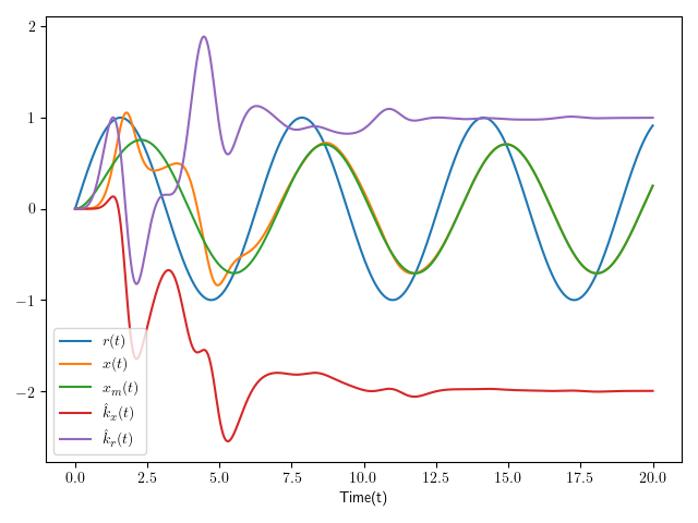
Figure 1: The simulation result for model reference adaptive control. Notice that \(e(t) = x(t) - x_m(t)\) converges to 0 and \(\hat k_x \rightarrow -2\) and \(\hat k_r \rightarrow 1\).