Table of Contents
- 1. Frequency Response
- 1.1. Introduction
- 1.2. What is Frequency Response: RC-Network
- 1.3. RC-Network: Step Response
- 1.4. RC-Network: Response to Sinusoidal Input with \(\omega = 5\)
- 1.5. RC-Network: Response to Sinusoidal Input with \(\omega = 50\)
- 1.6. Frequency Response
- 1.7. Why Do We Need Frequency Response
- 1.8. How to Get Frequency Response
- 1.9. How to get Frequency Response from Transfer Function
- 1.10. Example: RC-Network
- 1.11. RC-Network: Solution
- 1.12. Bode and Nyquist Plot
- 1.13. Bode Plot
- 1.14. Nyquist Plot
- 1.15. Real World Example: Voice Coil Motor
- 1.16. Hendrik Wade Bode(1905 - 1982)
- 1.17. Harry Nyquist (1889 - 1976)
- 1.18. Summary
1 Frequency Response
1.1 Introduction
Review of time domain analysis
- System modeling
- Time-domain responses systems of control
- Routh-Hurwitz Criterion and Root locus for stability analysis
- Time-domain specifications:
- rise time
- settling time
- maximum overshoot
- steady-state error
1.2 What is Frequency Response: RC-Network
Consider the above RC-network, whose transfer function is
\begin{align*} \frac{V_0(s)}{V_i(s)}= \frac{1/sC}{R+1/sC} = \frac{1}{\tau s+1},\,\tau=RC. \end{align*}Assuming \(R = 1k\Omega\), \(C = 10^{-4}F\), then \(\tau = 0.1s\).
1.3 RC-Network: Step Response
1.4 RC-Network: Response to Sinusoidal Input with \(\omega = 5\)
Assume the input is a sinusoidal wave:
\begin{align*} v_i(t) = 2\sin(5 t+ 30^\circ), \end{align*}
1.5 RC-Network: Response to Sinusoidal Input with \(\omega = 50\)
Assume the input is a sinusoidal wave:
\begin{align*} v_i(t) = 2\sin(50t+ 30^\circ), \end{align*}
1.6 Frequency Response
The frequency response of a system is defined as the steady-state response of the system to a sinusoidal input.
1.7 Why Do We Need Frequency Response
- The frequency response of a complex system can be derived from the response of simple systems (Bode Plot).
- The stability of the closed-loop system is determined by the frequency response of the open-loop system (Nyquist Stability Criterion)
- Controller design can be carried out in an intuitive fashion by shaping the frequency response of the open-loop systems (Lag, Lead, PID controller Design)
1.8 How to Get Frequency Response
- The frequency response can be derived from transfer functions
- The frequency response of complex systems can be obtained experimentally
- In fact, for an unknown system, usually we get its transfer function from the frequency response.
1.9 How to get Frequency Response from Transfer Function
Consider a stable system:
\begin{align*} G(s) = \frac{a(s)}{b(s)}=\frac{a(s)}{(s+p_1)\dots(s+p_n)}, \end{align*}where \(p_i\) are assumed to be distinct poles.
Consider the input
\begin{align*} r(t) = A \exp\left[j\omega t\right] = A\cos(\omega t + \phi)+jA\sin(\omega t+\phi). \end{align*}whose Laplace transform is
\begin{align*} R(s) = A\exp(j\phi)\frac{1}{s-j\omega}. \end{align*}The output is given by
\begin{align*} Y(s) &= G(s)R(s) \\ &= \frac{a(s)}{(s+p_1)\dots(s+p_n)}\times \frac{A\exp(j\phi)}{s-j\omega} \\ &=\frac{k_1}{s+p_1}+\frac{k_2}{s+p_2}+\dots+\frac{k_n}{s+p_n} + \frac{\alpha}{s-j\omega}. \end{align*}If we multiply the LHS and RHS of the equation by \(s-j\omega\) and take the limit \(s\rightarrow j\omega\), we get
\begin{align*} \lim_{s\rightarrow -j\omega}G(s)R(s) = A\exp(j\phi)G(j\omega) = A|G(j\omega)|\times e^{j(\phi + \angle G(j\omega))} = \alpha. \end{align*}Therefore, the response of the system can be written as
\begin{align*} y(t) &= k_1e^{-p_1t}+\dots+k_ne^{-p_nt} \\ &+ A|G(j\omega)|\cos(\omega t + \phi + \angle G(j\omega))\\ &+j A|G(j\omega)|\sin(\omega t + \phi + \angle G(j\omega)). \end{align*}If we input \(r(t) = A\sin(\omega t + \phi)\), then the steady-state output will be
\begin{align*} y_{ss}(t) = A|G(j\omega)|\sin(\omega t + \phi + \angle G(j\omega)). \end{align*}- The steady-state response of a sinusoidal signal is another sinusoidal signal, where
- The frequency is the same.
- The amplitude is \(A\times |G(j\omega)|\).
- The phase is \(\phi + \angle G(j\omega)\).
- \(|G (j\omega)|\) and \(\angle G(j\omega)\) are frequency dependent and are referred to as the magnitude and phase responses of the system, respectively.
1.10 Example: RC-Network
Consider the RC-network with transfer function
\begin{align*} G(s) = \frac{1}{0.1s+1}. \end{align*}Find the steady state output due to the input \(r(t) = 2\sin(\omega t+ 30^\circ)\).
1.11 RC-Network: Solution
- Notice that\[0.1j\omega + 1 = \sqrt{1+0.01\omega^2}\angle \tan^{-1}(0.1\omega).\]
- Therefore,\[G(j\omega) = \frac{1}{\sqrt{1+0.01\omega^2}}\angle -\tan^{-1}(0.1\omega).\]
- Hence, the response to \(r(t)\) is\[y_{ss}(t) = \frac{2}{\sqrt{1+0.01\omega^2}}\sin\left[\omega t+30^\circ -\tan^{-1}(0.1\omega)\right.\]
- For \(\omega = 5\), \(|G(j5)| = 0.8944\), \(\angle G(j5) = -26.6^\circ\).\[y_{ss}(t) = 1.7888\sin(5t+3.4^\circ).\]
- For \(\omega = 50\), \(|G(j5)| = 0.1961\), \(\angle G(j5) = -78.7^\circ\).\[y_{ss}(t) = 0.3922\sin(50t-48.7^\circ).\]
1.12 Bode and Nyquist Plot
- From the analysis above, \(G(j\omega)\) plays a key role in frequency response.
- To visualize \(G(j\omega)\), the following plots are typically used
- Bode Plots: Bode Magnitude Plot + Bode Phase Plot
- Nyquist Plots
1.13 Bode Plot
1.14 Nyquist Plot
1.15 Real World Example: Voice Coil Motor


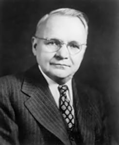
1.16 Hendrik Wade Bode(1905 - 1982)

- A pioneer of modern control theory and electronic telecommunications.
- He made important contributions to the design, guidance and control of anti-aircraft systems during World War II
- During the Cold War, he also made significant contributions to the design and control of missiles and anti-ballistic missiles.
- Contributions to control system theory and mathematical tools for the analysis of stability of linear systems, inventing Bode plots, gain margin and phase margin.
- Worked in Bell Lab from 1926 to 1967. Became a professor at Harvard after retiring from Bell Lab.
1.17 Harry Nyquist (1889 - 1976)
- Worked in Bell Lab from 1917 to 1954.
- Received the IEEE Medal of Honor in 1960 for "fundamental contributions to a quantitative understanding of thermal noise, data transmission and negative feedback."
- Received the National Academy of Engineering's fourth Founder's Medal "in recognition of his many fundamental contributions to engineering."
1.18 Summary
The frequency response of a system is defined as the steady-state response of the system to a sinusoidal input.
It is also a sinusoidal signal, where
- The frequency is the same.
- The amplitude is \(A\times |G(j\omega)|\).
- The phase is \(\phi + \angle G(j\omega)\).